
An inventory manager opens a replenishment screen on Monday morning. The AI supported system suggested order is 80 patio lanterns. There is enough budget to buy them, and the forecast comparison looks encouraging. Should the order go through? Before approving it, the manager needs to know which customers can actually receive stock, when the delivery arrives and what happens if demand falls short.
Retail analytics consulting can make those questions answerable. A forecast error chart helps establish whether a suggestion deserves attention. A dated stock calculation then shows whether the suggested quantity is useful. The purchase decision needs both.
Marlowe & Finch Home is a fictional two-store retailer used throughout this worked example. Its forecasts, stock records, costs and future dates are illustrative inputs; no AI model was trained or tested here. The figures explain a review method, not measured commercial results. In a real deployment, incomplete stock records, changing promotions, supplier delays and unobserved demand could change the decision.
Resource Toolkit
The accompanying retail analytics dashboard resource pack includes eight small CSV files, a calculation guide and four original figures. The files contain observed store-week sales, prior-season references, supplied forecasts, availability flags, reorder assumptions, demand scenarios and the resulting calculations. The final figure is a static buyer decision panel, rather than a live Power BI report.
What You’ll Learn
- Does the forecast comparison use the right periods and available-stock observations?
- Which affordable order remains useful when demand and arrival timing change?
- Who can approve the pilot, and what should pause the release?
Does the Forecast Comparison Support the Decision?
Start with the forecast’s purpose. The supplied comparison predicts one week of unit sales at each store. The order decision covers fourteen days. Those are different horizons: a useful weekly result cannot establish that a two-week replenishment suggestion is accurate.
For a real model, preserve the order of time when developing and evaluating it. Use earlier records to fit the model, a later window to choose settings, and an untouched final window to assess the chosen approach. The principle behind time series cross-validation is that forecasts use information available before the period being predicted. Future sales or a promotion outcome discovered afterward must not enter the earlier forecast.
Figure 1 shows a proposed chronological design. The final window runs from September 28 to November 1, 2026. It contains ten candidate store-weeks, but the first week has a stockout at each store. Those two rows are excluded from the accuracy calculation, leaving eight fully available observations from October 5 onward. No fitting exercise is represented by the timeline.
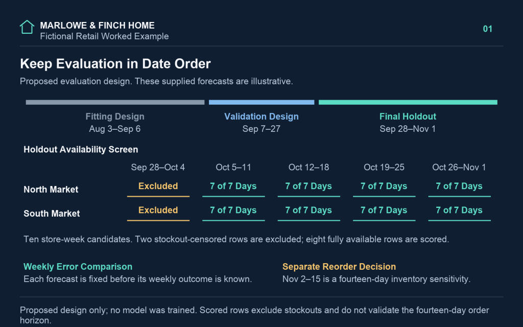
Figure 1. Proposed evaluation windows preserve chronology. Two stockout rows remain recorded but are excluded from the eight-row accuracy comparison.
That exclusion needs a careful explanation. Selling every available lantern does not tell the buyer how many more customers would have purchased one. Observed sales remain useful records, but unconstrained demand is unknown. The example leaves that field blank instead of inventing lost sales. Removing the rows also means the remaining accuracy result says nothing about performance during stockouts.
Compare both forecasts on those same eight rows. The baseline repeats each store’s observed sales from the corresponding week 52 weeks earlier. Its reference values are included in the pack, so the comparison can be rebuilt. A retailer would also check that last year’s availability, range and promotion conditions provide a sensible reference.
The supplied forecast has 45 units of total absolute error. Dividing by eight gives a mean absolute error of 5.625 units per store-week. The baseline totals 80 units of absolute error, giving 10.0. Mean absolute error describes the typical error size in the units being forecast.
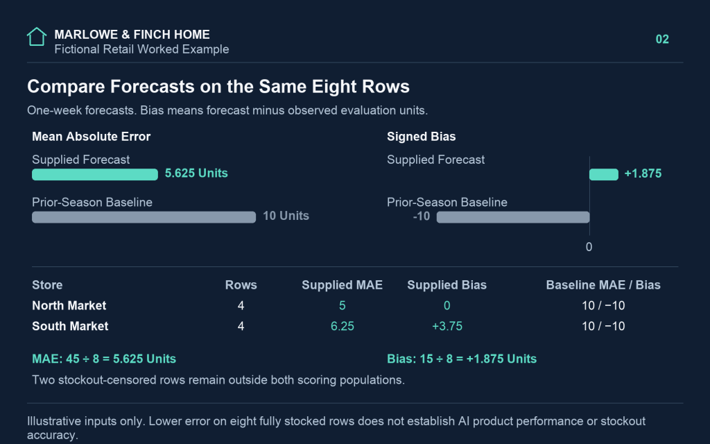
Figure 2. Both forecasts use the same eight fully available store-weeks. Positive bias here means forecast units exceed observed units.
Direction matters as well. Here, signed error means forecast minus observed units. The supplied values have a mean signed bias of +1.875 units, while the baseline has −10.0. North Market’s supplied errors cancel to zero on average; South Market’s bias is +3.75. The combined result therefore deserves a store-level look before the manager treats it as broadly representative.
These arithmetic results demonstrate the comparison, rather than establish an AI system’s superiority. Eight illustrative rows are too narrow to support a rollout claim. Before deployment, repeat the comparison on representative periods and on the fourteen-day horizon the buyer actually uses, including an appropriate way to assess demand when stock is unavailable.
Which Affordable Order Holds Up When Demand Changes?
Now consider North Market’s hypothetical decision on November 2. It holds 90 sellable lanterns, of which 20 are already reserved. That leaves 70 for additional demand. A confirmed, already-funded delivery of 30 arrives on November 9. Any new order arrives that morning too. The additional demand scenarios exclude the reserved commitments, so those customers are not counted twice.
New stock costs $12 per unit, comes in packs of 20 and has a $1,000 cash limit. The feasible quantities are therefore 0, 20, 40, 60 and 80 units. Buying 100 would cost $1,200 and break the limit. Check every feasible quantity: comparing only 0, 40 and 80 would miss the stronger candidate in this example.
Additional demand over November 2–15 is set at 100, 140 or 180 units. Each scenario places half before the deliveries arrive and half afterward. Unserved requests before arrival are lost; there are no backorders to recover later. This timing assumption is as consequential as the total demand.
The calculation assigns $8 of penalty cost to each unmet unit and $3 of assumed holding or markdown loss to each unit left at the horizon’s end. These are illustrative business inputs, not industry benchmarks. The $3 is a loss allowance, not the $12 purchase price. Retail markdown analysis helps explain why clearance economics need their own assumptions: remaining stock cannot simply be treated as if it would all sell at full price.
Figure 3 compares shortage-plus-excess penalty cost. It gives the three scenarios equal weight for sensitivity, without claiming that they are equally probable. The averages are $320.00, $233.33, $146.67, $133.33 and $193.33 for the five ascending order quantities. Under those assumptions, 60 units has the lowest average penalty cost and requires $720 of new-order cash.
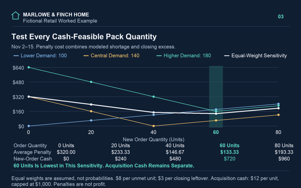
Figure 3. All five affordable pack quantities are compared. Equal scenario weights are a sensitivity assumption; penalty cost excludes purchase cash and full profit.
Walk through that 60-unit choice. In the lower case, 50 units sell before arrival, leaving 20. Adding the confirmed 30 and the new 60 creates 110 units for the remaining 50 requests. Sixty are left at the end, giving $180 of excess loss. The central case uses all 70 starting units before arrival, then sells 70 of the 90 received units. Its 20 leftovers create $60 of excess loss.
The higher case is more revealing. Ninety requests arrive before November 9, but only 70 units are available. Twenty requests are lost before either delivery arrives. Afterwards, the 30 confirmed units and the new 60 cover the remaining 90 requests exactly. The $160 penalty reflects the earlier shortage. Ordering 80 instead still loses those first 20 requests and then leaves 20 units unsold, raising that scenario’s penalty to $220.
A bigger order cannot repair an earlier missed sale. If avoiding that shortage is the priority, the manager needs a different operational option, such as a confirmed earlier delivery or a store transfer, with its own feasibility and cost calculation. Neither option is assumed in this example.
The comparison also does not calculate profit or return on investment. Purchase cash is shown separately; revenue, taxes and ordering costs are outside the penalty measure. A different demand split, a lower shortage penalty, or heavier emphasis on the central case could favor another quantity. The manager should challenge those inputs before treating 60 as a purchase instruction.
Who Can Release the Order and When Should It Pause?
The hypothetical tool suggests 80. The review proposes 60 for a bounded pilot at North Market, for this SKU and this fourteen-day window. Figure 4 keeps the proposed quantity beside available stock, arrival dates, cash use and the remaining shortage risk. The manager can see the reason for the override without opening several unrelated reports.
For teams commissioning data visualization consulting, the brief should specify units, dates, ownership and exception handling before visual styling. A Power BI consulting project should preserve those definitions when turning this static example into a refreshed report.
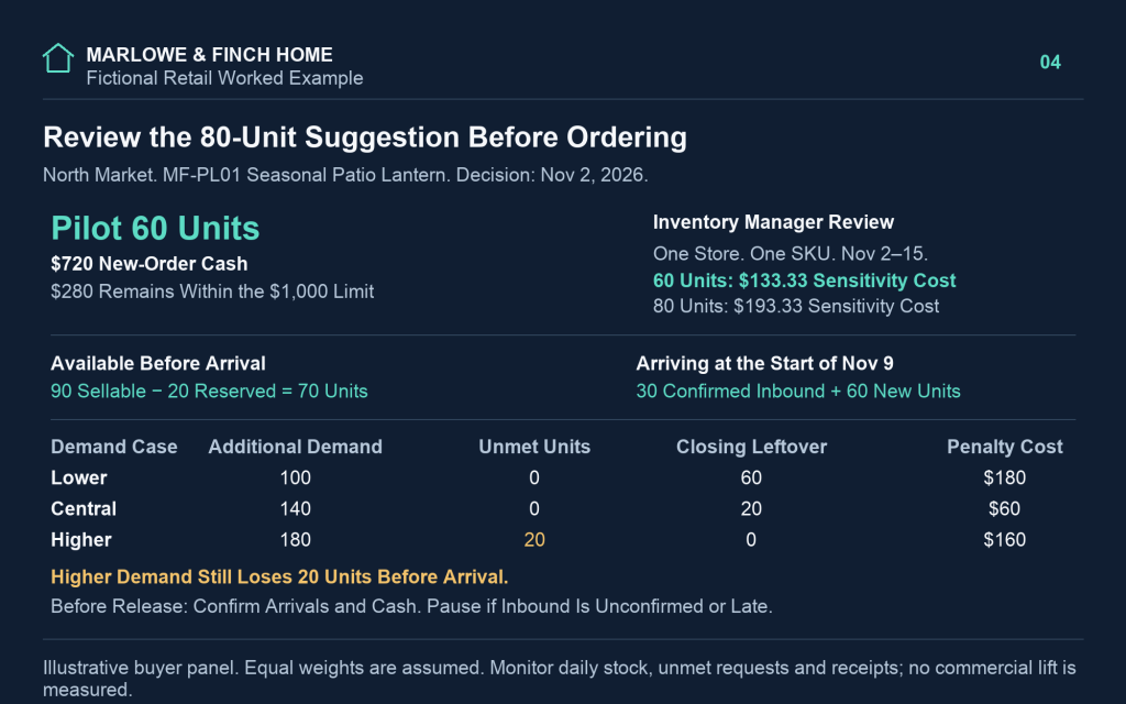
Figure 4. The illustrative static panel records a 60-unit pilot proposal, its owner, cash requirement and stop conditions. It does not authorize a live purchase.
Give the inventory manager authority to hold the release. Before ordering, confirm the inbound quantity, arrival date and reserved commitments. Pause if the delivery is unconfirmed, either arrival slips or the new-order cash exceeds $1,000. If the conditions change, recalculate the scenarios; yesterday’s comparison cannot approve a changed order.
During the pilot, record daily sellable stock, unmet requests and receipt status. Log the original suggestion, the manager’s chosen quantity, the reasons for changing it and the actual outcome. NIST’s AI risk management framework supports defined oversight roles, documented test conditions and monitoring during use. This example applies those ideas to a purchase review; it is not a certification of compliance.
At the end of the window, compare the outcome with the assumptions that drove approval. Did stock arrive on time? Were additional requests concentrated before arrival? Did the leftover units require a markdown? Keep supplier reliability, forecast error and managerial overrides visible as separate issues. A favorable outcome from one small trial is useful evidence for the next review, but does not justify removing the release controls across the whole range.
Keep the previous manual ordering policy as a dated comparator, with the same stock information and costs. Review the pilot alongside that alternative before expanding it. One favorable outcome cannot isolate the effect of the recommendation from demand changes or supplier performance.
The practical result is an order the buyer can question. Every quantity has a source, every trade-off has an assumption and somebody owns the release. That is the standard a retail team should expect before an AI recommendation commits its cash.
About the Author
Basem Fawzy is the founder of Data Pivot Consulting. He is a Microsoft Certified Power BI Developer and MBA graduate in E-Business with more than 10 years of experience in business intelligence, data modeling, dashboard development and reporting automation. He has worked with more than 200 clients and regularly translates operational data into management-level reporting frameworks.