Background: Counterfactuals and Causal Inference
At its core, causal inference is about “what if” questions, what would have happened if we hadn’t done X? So technically we put these questions through counterfactual analysis, for example, by considering the outcome in each single unit (treatment vs. control).
For estimating causal effects, we use comparisons of groups. For a perfectly randomized experiment (such as an A/B test), we ensure that the treatment and control groups are identical in the statistical expectation through random assignment. Therefore, the difference in average outcomes yields an unbiased estimation of the Average Treatment Effect (ATE): that is the average (Y(1)-Y(0)), that is, the mean in the population. But in many cases, we’re more likely to care for treated units than generalizations; the Average Treatment Effect on the Treated (ATT), also called ATET, measures the lift to participants who received the treatment. Functionally ATT = E[Y(1) – Y(0) ; T=1]. But outside of experiments, observational data are susceptible to selection bias. Maybe promoted users are naturally more likely to convert (high intent) than those who never received a promotion. In such a case, even naive comparison of outcomes would be biased due to pre-existing differences.
So, in fact a fundamental issue in observational studies is precisely this: Are users who view the ads/promotions more likely to buy even if nothing is done? If so, we might mischaracterize their greater conversion by attributing it to the campaign, when in fact it was a byproduct of their inherent propensity to convert. Counterfactual analysis offers a conceptual solution (compare each unit to its hypothetical self in the absence of treatment), while we lack the practical tools to approximate that with real data.
Propensity Score Matching and Its Limitations
Propensity Score Matching (PSM) is widely used to remove selection bias from observational studies. The goal is to resemble a randomized experiment and select treatment and control units which have similar probabilities of being treated using observed covariates. This probability is the propensity score, usually represented e(x) = P(T=1; X=x) in relation to the vector of pre-treatment features X. In real life, we estimate each unit’s propensity score (typically through a logistic regression or machine learning model) as the predicted probability of being in the treatment group based on its observed characteristics. This single score is an aggregation of all covariates. Rosenbaum and Rubin famously demonstrated that the degree to which treatment and control units have a common propensity score suggests they would ideally display similar distributions of all observed covariates like a propensity score a finding is a balancing score.
By matching one treated unit with one or more control units with close propensity score, PSM creates a matched sample with covariates more balanced between groups. This aids in estimating the counterfactual: the matched control is supposed to represent what the treated unit would have expected had it not received the treatment. We use the next example after matching to estimate the treatment effect, looking where outcomes differ between the matched treated and control units. For instance, ATT can be estimated by the average outcome difference between pairs of matched pairs. Using an appropriate formula, we can derive i as a treated unit and j(i) as its matched control, with j(i) being the matched control, and have the model predicting ATT through one-to-one matching
If i is a treated unit and j(i) is its matched control, an estimator for ATT via one-to-one matching is:
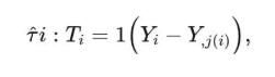
where N_T is the number of treated units. Intuitively, we look at the difference in outcome Y for each matched pair and average those differences for the treated group.
- Advantages: Confounding is lessened as we compare units with equivalent propensities. Instead of comparing a bunch of savvy repeat purchasers all of whom received a coupon against a random group of users who never received it, we compare each coupon-recipient with a very similar user who did not receive the coupon. It adjusts for observed covariates and increases group comparison, which is similar to conducting a randomized experiment. In other words, PSM is doing a kind of dimensionality reduction: matching on one score (the propensity) is easier and sometimes more effective than trying to match on too many attributes.
- Limitations: Propensity score methods can only account for observed confounders. If key variables have been omitted, or measured incorrectly, the matching won’t eliminate those biases. For example, if “user purchase history” plays a critical role in the decision of who receives a promotion and therefore affects the likelihood of purchasing a product, then failing to account for purchase history in the propensity model means that matched groups may still differ in their purchase history. Therefore, true PSM should be quality dependent on the propensity model and covariates used. A well-specified model containing all relevant features could even out those features across groups; poorly specified models may imply a false sense of safety.
There is also lack of overlap. So, if treated units have propensity scores much higher than any control (say all high-intent users got the coupon, low-intent did not), then there are areas of the feature space with no corresponding matches (this violates the common support assumption). PSM performs at its best when propensity score distributions overlap substantially. Always check balance diagnostics: Are the covariate means similar after matching? Are the differences in standardized mean differences small? Otherwise, matching might need to be further refined.
Lastly, when PSM balances out the observed covariates to some extent, residual bias may still exist if something like the baseline outcome differs. Importantly, in many circumstances, the baseline (before treatment) level of the outcome is a strong predictor of the outcome and often a confounding factor. PSM generally studies covariates X but there’s a particular covariate that is specifically relevant, which is the outcome itself at baseline, if it exists. That’s where target metric pre-balancing comes in.
Video: This video simulates how Treatment and Controls are matched based on Propensity score neighborhood
Pre-Balancing on the Target Metric
‘Pre-balancing’ your target metric means balancing the groups on the outcome measure of interest (or near-related measure), before you measure the effect of treatment. Put simply, you should compare treat or control groups at the baseline level of your target outcome. The intuition is simple: if we need to measure lift in conversion rate, we must determine whether any intrinsic conversion propensity is very similar between the treated and control groups at the beginning. This can significantly enhance match quality for the results and minimize selection bias attributable to differences in outcomes. Why is this important? To that, consider an e-commerce promotion that was pushed to regular shoppers. Those shoppers, for example, might have a 10% baseline conversion rate (for example, 1 in 10 visitors translates into a purchase) even without any promo, while the average user has a 2% baseline conversion rate. If we compare those two groups after the promotion, we’re not from a level playing field was much more “active”. If this baseline gap is not addressed, we will inflate our estimate for the promotion’s impact. From a technical point of view, the estimate of E[Y(0); T=1] (what the treated group would have done with no treatment) is greater than E[Y(0); T=0] for the untreated group, and that difference is entered into our effect estimate as a bias. Addition of baseline outcome as a confounder is the standard.
One strategy is to consider the prior outcome metric as a feature in our propensity model. For example, you might introduce a prediction of propensity to be targeted by the campaign from each user’s historical conversion rate (or purchase count, etc.). In doing so, you are not only matching on propensity score, but you are also indirectly matching on your baseline conversion propensity too (because propensity estimation factors this into it). And this often leads to much better balance on that metric. For our example, high-converting users that got the promo will be matched with high-converting users who didn’t, and low-converters matched with low-converters and so on. Or else, stratification or matching on the baseline metric.
One possibility would be to group users in groups across pre-existing conversion rates (e.g., low, medium or high) and make matching within each stratum. This ensures that a treated user and its matched control belong to the same conversion band at baseline. You’re just trying to make the matches match the corresponding (or near similar) baseline value and therefore pre-balance the target metric. This technique is a bit more like a one-way comparison to one another, for e.g. compare promo vs. no promo among users with ~2% baseline conversion vs users with ~10% baseline conversion. Then aggregate.
This pre-balancing on the target metric is to overcome the selection bias that happens via adverse selection on the outcome. A phenomenon that’s known in digital marketing as the “already converted” or “high intent” problem, means your treatment group is intentionally chosen to win. We mitigate this bias by adjusting for the baseline success probability. Indeed, practitioners tend to begin with baseline differences: if your treated group’s pre-campaign conversion or revenue is significantly higher than controls, you know that you must incorporate it into your causal inference. Simply to use formula terms, an observational difference in outcomes can be decomposed as:
The term selection bias usually comes from E[Y(0) | T=1] – E[Y(0) | T=0] i.e., in the absence of treatment the two groups would have yielded different outcomes. A pre-balancing on target metric is an attempt to ensure E[Y(0) | T=1] E[Y(0) | T=0] by equating a proxy for Y(0) (baseline outcome or model-predicted outcome) between groups. By doing so, the observed outcome difference after treatment is closer to the true treatment effect.
Use Case: Measuring a Promotional Campaign’s Impact on Conversion
Now, lets take an e-commerce example to illustrate these ideas. Let us assume an online retailer ran an email promotional campaign that gave a 20% discount offer to a subset of users (treatment group) to see if it caused more purchases from them. However, the campaign was not randomized – marketing has been aimed at users who, in past studies have shown high engagement levels (such as frequent browsers or past purchasers). We want to calculate the incremental conversion rate: how much did the promo actually increase the conversion rate compared to if those same users hadn’t received the promo? We must use observational methods since we do not have an ideal randomized control.
Problem Setup:
Treatment T=1: User received the promotional email
Control T=0: User did not receive the email
Outcome Y: Whether the customer/user made a purchase during the campaign (conversion = 1 or 0);
Key Covariates: User demographics, past behavior (e.g., prior purchase count, days since last purchase, browsing history), etc. Among these, a critical one is the user’s baseline conversion rate (before the campaign). We may measure this as the percentage of site visits that lead to a purchase for the user in the month leading up to the campaign, or it may even be just whether they bought that month before. It is a proxy for their natural disposition to convert.
So, considering the targeting strategy, we assume treated users have better baseline conversion rates than average users. In fact, if we were simply to look at the raw data ourselves, we might notice that the treated group had a 3% conversion rate during the campaign as opposed to 1% for a naive control group, which appears to indicate a +2% lift. But if the treated users’ baseline was, say, 2% vs. 0.5% of the control, then a lot of that lift is due to pre-existing differences (they were already converting more). We need to correct for that.
Applying Propensity Score Matching with Target-Metric Balancing:
In the code below, we begin with estimating propensity scores using an elastic net logistic regression (ElasticNetPropensityModel() from CausalML(). We had baseline_conversion_rate and some other confounders, among others. Once we have the propensity scores for each user, we append them to our DataFrame(). We next search for matches using NearestNeighborMatch() and note that we pass score_cols=[‘propensity_score’, ‘baseline_conversion_rate’].
This indicates to the matcher to take into account both the propensity and the baseline conversion rate when matching. In short, a treated-control pair will only match if they have similar propensity and similar baseline conversion. This is a method for enforcing target metric pre-balancing. (Or we could stratify according to baseline conversion groups with match_by_group(), it works the same).
Finally, we check balance with create_table_one(), which reports the mean value of each feature in treatment versus control groups and the standardized difference. We’d expect to find an almost identical baseline_conversion_rate() between the groups (std. diff ~ 0), which proves the successful pre-balancing, and it should tell us that the other features are balanced as well.
Results: Is Pre-Balancing Effective on Causal Estimates?
To demonstrate the effects of target metric pre-balancing, we compare outcomes in a hypothetical. We reproduce an observational study where baseline conversion rate in the treated group is a lot higher than that in the control group and a true causal lift from the treatment of several percentage points is real. We then obtain the ATT from three ways:
- no matching (raw difference),
- propensity score matching without baseline conversion being used as the covariate, and
- propensity score matching plus baseline conversion included (pre-balanced).
The table below summarizes the results (to illustrate it by number)
| Method | Treated baseline | Control baseline | Treated outcome | Control outcome | Estimated lift (diff) |
| Unmatched (Raw) | 38.7% | 26.0% | 44.8% | 26.4% | 18.4% |
| PSM (no baseline) | 38.6% | 25.2% | 44.5% | 25.7% | 18.9% |
| PSM (with baseline) | 35.7% | 35.7% | 41.8% | 37.2% | 4.6% |
Unmatched (Raw) The users treated had a baseline conversion rate of around 38.7%, compared to 26.0% for controls, and at the campaign time their recorded conversion was 44.8% vs 26.4%. The naive lift estimate would be 18.4 points. But a lot of that is bias: treated users began ~12.7 points higher in baseline conversion. We can see that PSM without baseline did not do much to remedy this – the baseline gap remains the same, ~13.4 points up; and the estimated lift (~18.9 points) is nearly the same (even slightly above).
This held true because the propensity model neglected to include the major confounder, causing matching to not match up users with similar baseline propensities; treated high-converters were matched to controls (who tended to be lower-converters) without controlling for bias. By comparison, PSM with baseline pre-balancing had the same baseline conversion rate as the data for users when comparing to pretreatment-baseline rates 35.7% vs 35.7% for the treated vs control). The conversion rates for the outcomes at that time were 41.8% against 37.2% with lift estimated at ~4.6 points. This closely approximates to the real lift built into the simulation (which this time was 5%).
That is, we dramatically decreased the overestimation by making the treated and control groups as likely as the others to convert at baseline. The large apparent boost in the raw data was also largely selection bias; we recover considerably smaller (the realistic) causal effect after pre-balancing. For treated vs. control, baseline conversion rate distributions prior to matching (left) and after matching using target metric pre-balancing (right). The pre-balancing will provide a common baseline conversion distribution and thus remove one of the largest sources of bias of the treated and control groups.
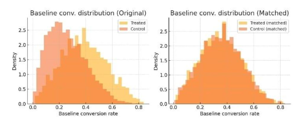
The figure above visualizes the difference. Initially, the treated group’s baseline conversion rate is skewed higher (blue curve vs. orange curve, left panel). After matching on propensity and baseline, the distributions overlap almost perfectly (right panel). This is evidence that our matching succeeded in creating apples-to-apples comparisons. As a result, the difference in outcomes can more credibly be attributed to the treatment (promo) itself, not to pre-existing differences.
Conclusion
The next big implication is that causal inference in data science often involves assembling a plausible control group from observational data. Propensity score matching helps to replicate a controlled experiment by taking into account the observed confounders between treated and untreated groups. But as we previously indicated, not all confounders are equal – the target outcome’s previous value is usually very important. Target metric pre-balancing (such as baseline conversion rates) is a method to ensure comparison of apples to apples and is particularly relevant to e-commerce, given the high heterogeneity of user behavior. Pre-balancing the outcome measure minimizes the selection bias and hence improves the quality of results at the level of estimates of the causal relationship.
The e-commerce example illustrated it all, if we don’t carefully balance this, estimated lifts get artificially inflated, while an exercise in balancing, on the other hand, brings back the actual incremental impact of an intervention. The outcome is more reliable insight: we can answer confidently how much a promotion produced an increase in conversions, rather than misunderstanding a distinction that was present for a causal effect.
For data scientists, the biggest takeaway is to always be mindful of what is ultimately driving your result. Do that for your matching or weighting. Use libraries like CausalML() or DoWhy() to assist with implementation – but keep in mind there’s no way that the library can understand what you left out. In causal learning, knowledge of one domain (the understanding, for example, that past conversion behavior is important) combined with statistical tools will yield the best outcome. Pre-balancing target metrics is one type of standard technique in which that knowledge significantly builds upon and enriches. With these insights, you can ask more specific causal questions in e-commerce and elsewhere, more confidently and accurately.
Author: Dharmateja Priyadarshi Uddandarao
Dharmateja Priyadarshi Uddandarao is an accomplished data scientist and statistician, recognized for integrating advanced statistical methods with practical economic applications. He has led projects at leading technology companies, including Capital One and Amazon, applying complex analytical techniques to address real-world challenges. He currently serves as a Senior Data Scientist–Statistician at Amazon.