
Machine learning, a crucial subset of artificial intelligence, enables systems to learn from data, identify patterns, and make decisions with minimal human intervention. This transformative technology is revolutionizing industries such as healthcare and finance by enhancing data-driven decision-making processes. As machine learning techniques become increasingly complex, accessing quality assignment help from services like AssignmentCore is vital for both students and professionals to deepen their understanding and application of these methodologies.

Supervised Learning: Algorithms and Applications
Supervised learning involves training a model on a labeled dataset, which includes input-output pairs, enabling the model to make predictions based on this training. This section explores common supervised learning algorithms and their applications:
Linear Regression
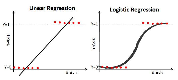
Linear regression is used to predict continuous outcomes by establishing a relationship between a dependent variable and one or more independent variables through a linear equation. Understanding this concept is fundamental for many machine-learning tasks. Below is an example to illustrate how a linear regression model is constructed and visualized.
A scatter plot with a regression line showing the relationship between the independent variable (X) and the dependent variable (Y). The plot should include data points, the best-fit line, and the equation of the line.
Example:
import matplotlib.pyplot as plt
import numpy as np
# Example data
X = np.array([1, 2, 3, 4, 5])
Y = np.array([2, 3, 5, 7, 11])
# Fit line
coef = np.polyfit(X, Y, 1)
poly1d_fn = np.poly1d(coef)
plt.scatter(X, Y, color=’blue’, label=’Data Points’)
plt.plot(X, poly1d_fn(X), color=’red’, label=’Best Fit Line’)
plt.xlabel(‘Independent Variable (X)’)
plt.ylabel(‘Dependent Variable (Y)’)
plt.title(‘Linear Regression Model’)
plt.legend()
plt.show()
Logistic Regression
Logistic regression is essential for binary classification problems, modeling the probability of a certain class or event. Understanding how logistic regression differs from linear regression, the role of the sigmoid function, and how to evaluate the model’s performance are crucial skills. Here’s an example that visualizes the sigmoid function used in logistic regression.
A graph showing the sigmoid curve of logistic regression. This figure should illustrate how the probability output maps to the binary classification (0 or 1) depending on the threshold.
Example:
import matplotlib.pyplot as plt
import numpy as np
# Sigmoid function
def sigmoid(x):
return 1 / (1 + np.exp(-x))
# Example data
X = np.linspace(-10, 10, 100)
Y = sigmoid(X)
plt.plot(X, Y, color=’green’)
plt.axhline(0.5, color=’red’, linestyle=’–‘, label=’Threshold (0.5)’)
plt.xlabel(‘Input Feature’)
plt.ylabel(‘Probability’)
plt.title(‘Logistic Regression Sigmoid Curve’)
plt.legend()
plt.show()
Decision Trees
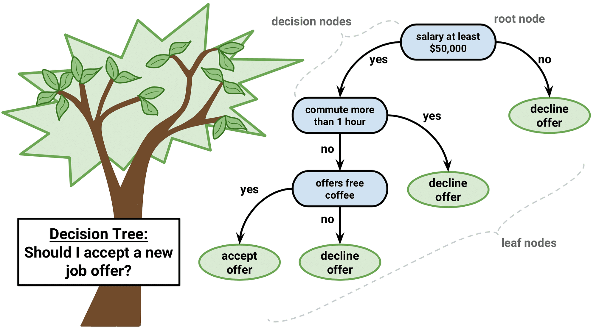
Decision trees are intuitive models that split the data into branches to form a tree-like structure of decisions, making them useful for both classification and regression tasks. Here’s an example that demonstrates how to create and visualize a decision tree.
A visual representation of a decision tree with nodes and branches. This should include decision nodes (internal nodes), leaf nodes (end nodes), and the conditions or rules at each node.
Example:
from sklearn.tree import DecisionTreeClassifier
from sklearn import tree
import matplotlib.pyplot as plt
# Example data
X = [[0, 0], [1, 1]]
Y = [0, 1]
# Fit decision tree
clf = DecisionTreeClassifier().fit(X, Y)
# Plot tree
plt.figure(figsize=(10, 8))
tree.plot_tree(clf, filled=True, feature_names=[‘Feature 1’, ‘Feature 2’], class_names=[‘Class 0’, ‘Class 1’])
plt.title(‘Decision Tree Structure’)
plt.show()
Support Vector Machines (SVM)
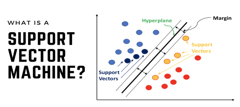
Support Vector Machines (SVMs) are powerful tools for classification tasks, finding the hyperplane that best separates classes in the feature space. Understanding kernel functions, margin maximization, and handling non-linear data are crucial. Here’s an example illustrating how to implement and visualize an SVM model.
A plot showing data points of two classes, the hyperplane that separates them, and the support vectors. This figure can also include margins on either side of the hyperplane.
Example:
import matplotlib.pyplot as plt
import numpy as np
from sklearn import svm
# Example data
X = np.array([[2, 3], [3, 4], [4, 5], [1, 1], [2, 1], [3, 2]])
Y = [1, 1, 1, 0, 0, 0]
# Fit SVM
clf = svm.SVC(kernel=’linear’, C=1.0)
clf.fit(X, Y)
# Plot
plt.scatter(X[:, 0], X[:, 1], c=Y, s=30, cmap=plt.cm.Paired)
# Plot decision boundary
ax = plt.gca()
xlim = ax.get_xlim()
ylim = ax.get_ylim()
xx = np.linspace(xlim[0], xlim[1], 30)
yy = np.linspace(ylim[0], ylim[1], 30)
YY, XX = np.meshgrid(yy, xx)
xy = np.vstack([XX.ravel(), YY.ravel()]).T
Z = clf.decision_function(xy).reshape(XX.shape)
ax.contour(XX, YY, Z, colors=’k’, levels=[-1, 0, 1], alpha=0.5, linestyles=[‘–‘, ‘-‘, ‘–‘])
# Plot support vectors
ax.scatter(clf.support_vectors_[:, 0], clf.support_vectors_[:, 1], s=100, linewidth=1, facecolors=’none’, edgecolors=’k’)
plt.title(‘Support Vector Machine’)
plt.xlabel(‘Feature 1’)
plt.ylabel(‘Feature 2’)
plt.show()
Unsupervised Learning: Discovering Hidden Patterns
Unsupervised learning deals with unlabeled data, focusing on identifying hidden patterns or intrinsic structures within the input data. This section covers essential unsupervised learning techniques such as clustering and Principal Component Analysis (PCA).
Clustering
Clustering algorithms, such as K-means, group similar data points together, making them essential for tasks like market segmentation and image compression. Here’s an example demonstrating how to implement and visualize K-means clustering.
A scatter plot showing data points colored by their cluster assignments. Cluster centers are marked with distinct symbols.
import matplotlib.pyplot as plt
from sklearn.cluster import KMeans
import numpy as
Principal Component Analysis (PCA)
PCA reduces the dimensionality of data, highlighting its most important features. It is widely used in data visualization and noise reduction. Experts can assist you online in comprehending and applying PCA effectively. They can explain eigenvalues and eigenvectors and how to interpret the principal components.
A scatter plot showing the original high-dimensional data points projected onto the first two principal components.
import matplotlib.pyplot as plt
from sklearn.decomposition import PCA
# Example data
X = np.array([[2.5, 2.4], [0.5, 0.7], [2.2, 2.9], [1.9, 2.2], [3.1, 3.0], [2.3, 2.7], [2, 1.6], [1, 1.1], [1.5, 1.6], [1.1, 0.9]])
# Fit PCA
pca = PCA(n_components=2)
principalComponents = pca.fit_transform(X)
# Plot
plt.scatter(principalComponents[:, 0], principalComponents[:, 1], color=’blue’)
plt.title(‘Principal Component Analysis (PCA)’)
plt.xlabel(‘Principal Component 1’)
plt.ylabel(‘Principal Component 2’)
plt.show()

Association Rules
Association rules are used for market basket analysis. They identify interesting correlations and associations within large datasets. Online help from machine learning experts can make these concepts clear and actionable. They can help you understand support, confidence, and lift, as well as how to implement association rule mining algorithms like Apriori.
Reinforcement Learning: Dynamic Decision Making
Reinforcement learning involves training agents to make a sequence of decisions by rewarding desired actions. It is highly effective in scenarios requiring complex decision-making, such as game playing and robotic control.
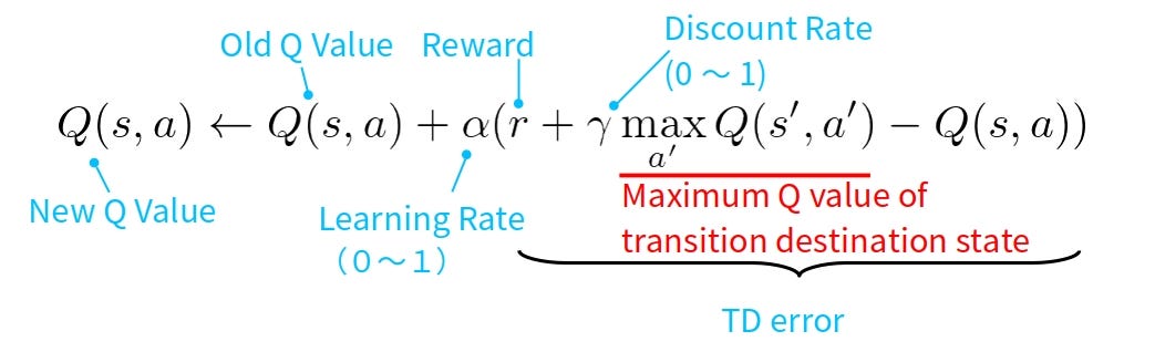
Q-Learning
Q-learning is a model-free reinforcement learning algorithm. It seeks to learn the quality of actions, informing the agent of the best actions to take in various states. Experts can offer detailed online assistance to help you master Q-learning. They can guide you through understanding the Q-value function, the exploration-exploitation trade-off, and how to implement Q-learning in practical scenarios.
A flowchart showing the Q-learning process, including states, actions, rewards, and updating Q-values.
graph TD
A[Start State] –> B[Take Action]
B –> C[Receive Reward]
C –> D[Update Q-Value]
D –> E[Next State]
E –> B
Deep Reinforcement Learning
Combining reinforcement learning with deep learning, this technique enables agents to handle high-dimensional inputs. It has been successful in tasks like playing video games and autonomous driving. Online experts are available to provide comprehensive machine learning assignment help in this advanced area. They can explain deep Q-networks (DQNs), policy gradients, and how to train these models effectively.
Model Evaluation and Validation
To ensure the reliability and accuracy of a machine learning model, thorough evaluation and validation are crucial.
Cross-Validation
Cross-validation assesses the performance of a model by dividing data into training and testing subsets multiple times. This provides a more accurate measure of model performance. Online experts can guide you through cross-validation techniques for your assignments. They can help you understand k-fold cross-validation, stratified sampling, and how to interpret cross-validation results.
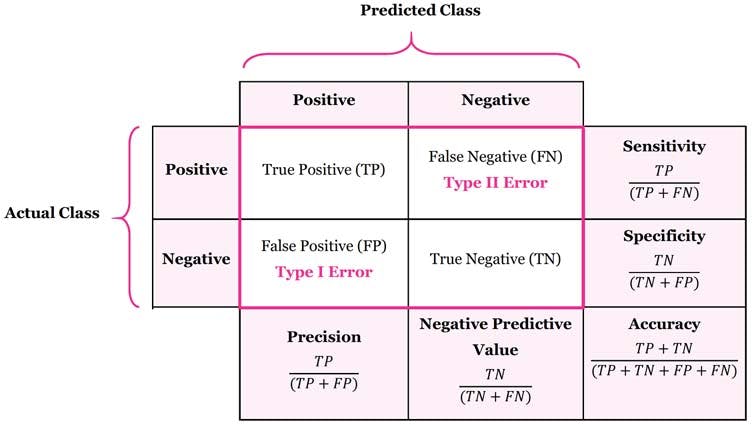
Confusion Matrix
A confusion matrix is used to evaluate the accuracy of a classification model. It shows the true positive, false positive, true negative, and false negative predictions. Machine learning assignment help from experts can make this concept easier to understand and apply. They can explain how to calculate and interpret precision, recall, F1-score, and overall accuracy from a confusion matrix.
A matrix visualization showing the true positives, false positives, false negatives, and true negatives for a classification model.
import matplotlib.pyplot as plt
import seaborn as sns
from sklearn.metrics import confusion_matrix
# Example data
y_true = [0, 1, 0, 1, 0, 1, 1, 0, 0, 1]
y_pred = [0, 1, 0, 0, 0, 1, 1, 0, 1, 1]
# Compute confusion matrix
cm = confusion_matrix(y_true, y_pred)
# Plot confusion matrix
sns.heatmap(cm, annot=True, fmt=’d’, cmap=’Blues’, xticklabels=[‘Predicted 0’, ‘Predicted 1’], yticklabels=[‘Actual 0’, ‘Actual 1’])
plt.title(‘Confusion Matrix’)
plt.xlabel(‘Predicted Label’)
plt.ylabel(‘True Label’)
plt.show()
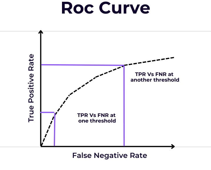
ROC and AUC
The Receiver Operating Characteristic (ROC) curve and the Area Under the Curve (AUC) are metrics for evaluating classification models. They measure the trade-off between the true positive rate and the false positive rate. Online assistance from experts can enhance your understanding of these evaluation metrics. They can show you how to plot ROC curves, calculate AUC, and use these metrics to compare different models.
A plot showing the ROC curve with the true positive rate (sensitivity) against the false positive rate (1-specificity) at various threshold settings.
import matplotlib.pyplot as plt
from sklearn.metrics import roc_curve, auc
# Example data
y_true = [0, 1, 0, 1, 0, 1, 1, 0, 0, 1]
y_scores = [0.1, 0.9, 0.2, 0.8, 0.1, 0.85, 0.95, 0.4, 0.3, 0.75]
# Compute ROC curve
fpr, tpr, _ = roc_curve(y_true, y_scores)
roc_auc = auc(fpr, tpr)
# Plot ROC curve
plt.figure()
plt.plot(fpr, tpr, color=’darkorange’, lw=2, label=f’ROC curve (area = {roc_auc:.2f})’)
plt.plot([0, 1], [0, 1], color=’navy’, lw=2, linestyle=’–‘)
plt.xlim([0.
Ethical Considerations in Machine Learning
As machine learning becomes more integrated into society, ethical considerations are paramount. Ensuring fairness, accountability, and transparency in algorithms is essential.
Bias and Fairness
Algorithms can inadvertently perpetuate biases present in training data. It is critical to address these biases to ensure fair outcomes. Online experts can help you navigate the complexities of bias and fairness in your machine-learning assignments. They can provide insights into detecting bias, debiasing techniques, and promoting fairness in model development.
Privacy
Protecting user data privacy is crucial. Techniques like differential privacy help in maintaining data confidentiality while enabling analysis. Machine learning assignment help can ensure you understand and implement these privacy-preserving techniques. Experts can explain how to balance data utility with privacy, implement anonymization techniques, and comply with data protection regulations.
Accountability
Ensuring that machine learning systems are accountable for their decisions is important. This involves clear documentation and an understanding of how models make decisions. Experts can provide online assistance to help you ensure accountability in your machine-learning projects. They can guide you in creating transparent models, documenting the decision-making process, and ensuring the reproducibility of results.
Conclusion
Machine learning is a rapidly evolving field with vast potential to transform industries. By understanding and applying advanced techniques, we can build robust, accurate, and fair models that drive innovation and efficiency. With the support of online experts and comprehensive machine learning assignment help, you can excel in this transformative field.