

One day, a friend of mine told me that the key to financial freedom is investing in stocks which got me thinking about stock analysis.
While it is greatly true during the market boom, it still remains an attractive option today to trade stocks part-time. Given the easy access to online trading platforms, there are many self-made value investors or housewife traders. There are even success stories and advertisements which boast “Get Rich Quick Scheme” to learn how to invest in stocks with a staggering return of 40% and even more.
Investing has become the boon for the working professionals today.
The question now is: Which stocks? How do you analyse stocks? What are the returns and risks of these stocks compared to their competitors?
The objective of this publication is for you to understand one way of analyzing stocks using a quick and dirty Python Code. Just spend 12 minutes to read this article — or even better, contribute. Then you could get a quick glimpse to code your first financial analysis.
To start learning and analyzing stocks, we will start off by taking a quick look at the historical stock prices. This will be done by extracting the latest stock data from pandas web-data reader and Yahoo Finance. Then we will try to view the data through exploratory analysis such as correlation heatmap, matplotlib visualization, and prediction analysis using Linear Analysis and K Nearest Neighbor (KNN).
Loading YahooFinance Dataset
Pandas web data reader is an extension of the pandas’ library to communicate with most updated financial data. This will include sources such as Yahoo Finance, Google Finance, Enigma, etc.
We will extract Apple’s Stock Price using the following codes:
import pandas as pd
import datetime
import pandas_datareader.data as web
from pandas import Series, DataFrame


start = datetime.datetime(2010, 1, 1)
end = datetime.datetime(2017, 1, 11)

df = web.DataReader("AAPL", 'yahoo', start, end)
df.tail()
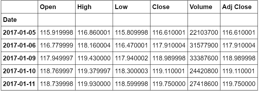
This piece of code will pull 7 years of data from January 2010 until January 2017 to give us the start of our stock analysis. Feel free to tweak the start and end date as you see necessary. For the rest of the analysis, we will use the Closing Price which remarks the final price in which the stocks are traded by the end of the day.
Exploring Rolling Mean and Return Rate of Stocks
In this analysis, we analyse stocks using two key measurements: Rolling Mean and Return Rate.
Rolling Mean (Moving Average) — to determine the trend
Rolling mean/Moving Average (MA) smooths out price data by creating a constantly updated average price.
This is useful to cut down “noise” in our price chart. Furthermore, this Moving Average could act as “Resistance” meaning from the downtrend and uptrend of stocks you could expect it will follow the trend and less likely to deviate outside its resistance point.
Let’s start code out the Rolling Mean:
close_px = df['Adj Close']mavg = close_px.rolling(window=100).mean()
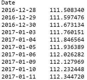
This will calculate the Moving Average for the last 100 windows (100 days) of the stock closing price and take the average for each of the window’s moving average. As you could see, The Moving Average steadily rises over the window and does not follow the jagged line of the stock price chart.
For better understanding, let’s plot it out with Matplotlib. We will overlay the Moving Average with our Stocks Price Chart.
%matplotlib inline
import matplotlib.pyplot as plt
from matplotlib import style

# Adjusting the size of matplotlib
import matplotlib as mpl
mpl.rc('figure', figsize=(8, 7))
mpl.__version__

# Adjusting the style of matplotlib
style.use('ggplot')

close_px.plot(label='AAPL')
mavg.plot(label='mavg')
plt.legend()
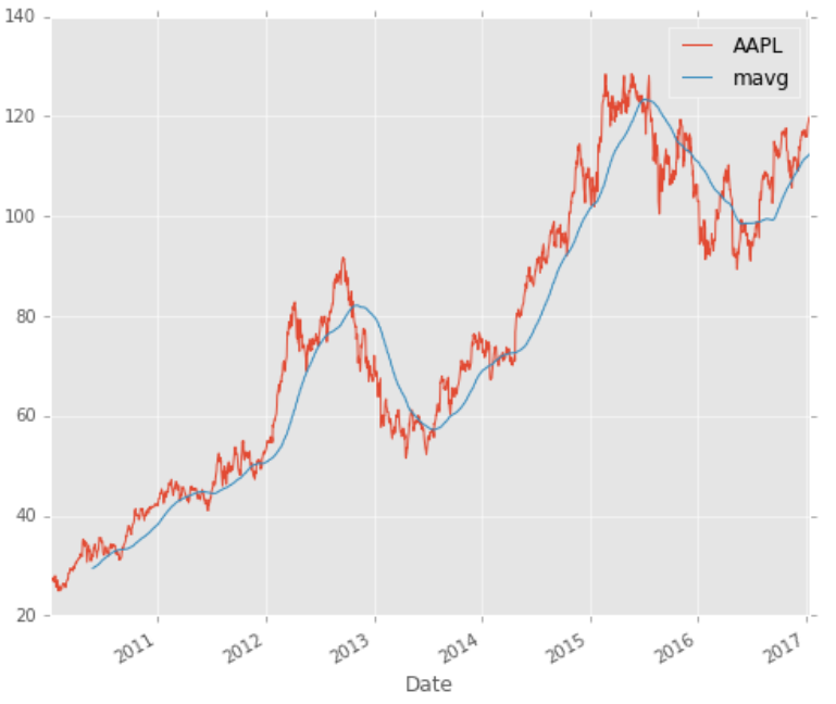
The Moving Average makes the line smooth and showcase the increasing or decreasing trend of a stock price.
In this chart, the Moving Average showcases the increasing trend in the upturn or downturn of a stock price. Logically, you should buy when the stocks are experiencing a downturn and sell when the stocks are experiencing an upturn.
Return Deviation — to determine risk and return in stock analysis
Expected Return measures the mean, or expected value, of the probability distribution of investment returns. The expected return of a portfolio is calculated by multiplying the weight of each asset by its expected return and adding the values for each investment — Investopedia.
Following is the formula you could refer to:
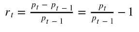
Based on the formula, we could plot our returns as follows.
rets = close_px / close_px.shift(1) - 1rets.plot(label='return')
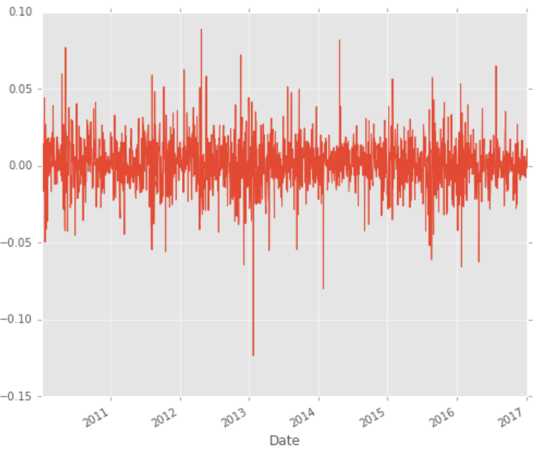
Logically, our ideal stocks should return as high and stable as possible. If you are risk-averse(like me), you might want to avoid these stocks as you saw the 10% drop in 2013. This decision is heavily subjected to your general sentiment of the stocks and competitor analysis.
Competitor Stock Analysis
In this segment, we are going to analyse on how one company performs relative with its competitor. Let’s assume we are interested in technology companies and want to compare the big guns: Apple, GE, Google, IBM, and Microsoft.
dfcomp = web.DataReader(['AAPL', 'GE', 'GOOG', 'IBM', 'MSFT'],'yahoo',start=start,end=end)['Adj Close']

This will return you a slick table of closing prices among the stock prices from Yahoo Finance. Neat!
Correlation Analysis — Does one competitor affect others?
We can analyse the competition by running the percentage change and correlation function in pandas. Percentage change will find how much the price changes compared to the previous day which defines returns. Knowing the correlation will help us see whether the returns are affected by other stocks’ returns
retscomp = dfcomp.pct_change()

corr = retscomp.corr()
Let’s plot Apple and GE with ScatterPlot to view their return distributions.
plt.scatter(retscomp.AAPL, retscomp.GE)
plt.xlabel(‘Returns AAPL’)
plt.ylabel(‘Returns GE’)
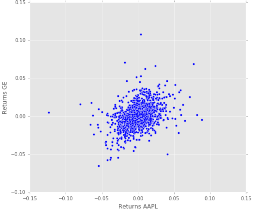
We can see here that there are slight positive correlations among GE returns and Apple returns. It seems like the higher the Apple returns, the higher GE returns as well for most cases.
Let us further improve our analysis by plotting the scatter_matrix to visualize possible correlations among competing stocks. At the diagonal point, we will run a Kernel Density Estimate (KDE).
KDE is a fundamental data smoothing problem where inferences about the population are made, based on a finite data sample. It helps generate estimations of the overall distributions.
pd.scatter_matrix(retscomp, diagonal='kde', figsize=(10, 10));
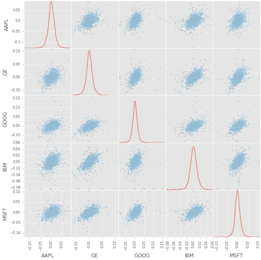
From here we could see most of the distributions among stocks which approximately positive correlations.
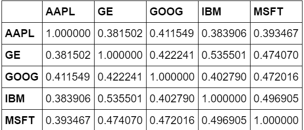
To prove the positive correlations, we will use heat maps to visualize the correlation ranges among the competing stocks. Notice that the lighter the color, the more correlated the two stocks are.
plt.imshow(corr, cmap='hot', interpolation='none')
plt.colorbar()
plt.xticks(range(len(corr)), corr.columns)
plt.yticks(range(len(corr)), corr.columns);
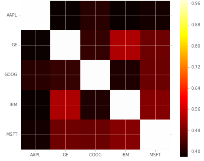
From the Scatter Matrix and Heatmap, we can find great correlations among the competing stocks. However, this might not show causality, and could just show the trend in the technology industry rather than show how competing stocks affect each other.
Stocks Returns Rate and Risk
Apart from correlation, we also analyse each stock’s risks and returns. In this case, we are extracting the average returns (Return Rate) and the standard deviation of returns (Risk).
plt.scatter(retscomp.mean(), retscomp.std())
plt.xlabel('Expected returns')
plt.ylabel('Risk')
for label, x, y in zip(retscomp.columns, retscomp.mean(), retscomp.std()):
    plt.annotate(
        label,
        xy = (x, y), xytext = (20, -20),
        textcoords = 'offset points', ha = 'right', va = 'bottom',
        bbox = dict(boxstyle = 'round,pad=0.5', fc = 'yellow', alpha = 0.5),
        arrowprops = dict(arrowstyle = '->', connectionstyle = 'arc3,rad=0'))
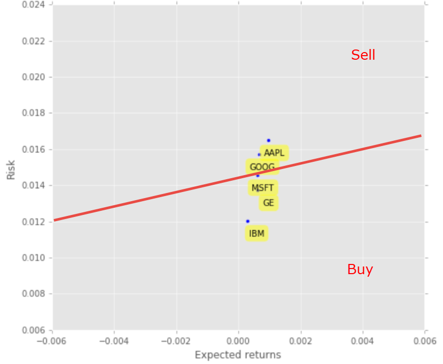
Now you could view this neat chart of risk and return comparisons for competing stocks. Logically, you would like to minimize the risk and maximize returns. Therefore, you would want to draw the line for your risk-return tolerance (The red line). You would then create the rules to buy those stocks under the red line (MSFT, GE, and IBM) and sell those stocks above the red line (AAPL and GOOG). This red line showcases your expected value threshold and your baseline for buy/sell decision.
Predicting Stocks Price
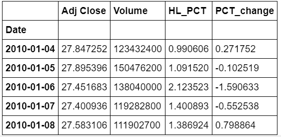
Feature Engineering
We will use these three machine learning models to predict our stocks: Simple Linear Analysis, Quadratic Discriminant Analysis (QDA), and K Nearest Neighbor (KNN). But first, let us engineer some features: High Low Percentage and Percentage Change.
dfreg = df.loc[:,[‘Adj Close’,’Volume’]]dfreg[‘HL_PCT’] = (df[‘High’] — df[‘Low’]) / df[‘Close’] * 100.0
dfreg[‘PCT_change’] = (df[‘Close’] — df[‘Open’]) / df[‘Open’] * 100.0
Pre-processing and Cross-Validation in stock analysis
We will clean up and process the data using the following steps before putting them into the prediction models:
- Drop missing value
- Separating the label here, we want to predict the AdjClose
- Scale the X so that everyone can have the same distribution for linear regression
- Finally, We want to find Data Series of late X and early X (train) for model generation and evaluation
- Separate label and identify it as y
- Separation of training and testing of the model by cross-validation train test split
Please refer to the preparation codes below.
# Drop missing value
dfreg.fillna(value=-99999, inplace=True)# We want to separate 1 percent of the data to forecast
forecast_out = int(math.ceil(0.01 * len(dfreg)))# Separating the label here, we want to predict the AdjClose
forecast_col = 'Adj Close'
dfreg['label'] = dfreg[forecast_col].shift(-forecast_out)
X = np.array(dfreg.drop(['label'], 1))# Scale the X so that everyone can have the same distribution for linear regression
X = preprocessing.scale(X)# Finally We want to find Data Series of late X and early X (train) for model generation and evaluation
X_lately = X[-forecast_out:]X = X[:-forecast_out]# Separate label and identify it as y
y = np.array(dfreg['label'])
y = y[:-forecast_out]
Model Generation — Where the prediction fun starts in stock analysis
But first, let’s insert the following imports for our Scikit-Learn:
from sklearn.linear_model import LinearRegression
from sklearn.neighbors import KNeighborsRegressor

from sklearn.linear_model import Ridge
from sklearn.preprocessing import PolynomialFeatures
from sklearn.pipeline import make_pipeline
Simple Linear Analysis and Quadratic Discriminant Analysis
Simple Linear Analysis shows a linear relationship between two or more variables. When we draw this relationship within two variables, we get a straight line. Quadratic Discriminant Analysis would be similar to Simple Linear Analysis, except that the model allowed polynomial (e.g: x squared) and would produce curves.
Linear Regression predicts dependent variables (y) as the outputs are given independent variables (x) as the inputs. During the plotting, this will give us a straight line as shown below:
This is an amazing publication that showed a very comprehensive review of Linear Regression. Please refer to this link for the view.
We will plug and play the existing Scikit-Learn library and train the model by selecting our X and y train sets. The code will be as follows.
# Linear regression
clfreg = LinearRegression(n_jobs=-1)
clfreg.fit(X_train, y_train)# Quadratic Regression 2
clfpoly2 = make_pipeline(PolynomialFeatures(2), Ridge())
clfpoly2.fit(X_train, y_train)

# Quadratic Regression 3
clfpoly3 = make_pipeline(PolynomialFeatures(3), Ridge())
clfpoly3.fit(X_train, y_train)
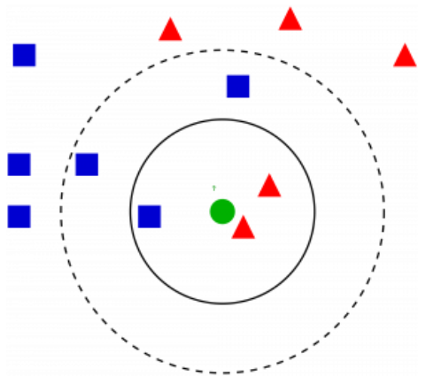
K Nearest Neighbor (KNN)
This KNN uses feature similarity to predict the values of data points. This ensures that the new point assigned is similar to the points in the data set. To find out the similarity, we will extract the points to release the minimum distance (e.g: Euclidean Distance).
Please refer to this link for further details on the model. This is really useful to improve your understanding.
# KNN Regression
clfknn = KNeighborsRegressor(n_neighbors=2)
clfknn.fit(X_train, y_train)
Evaluation
A simple quick and dirty way to evaluate is to use the scoring method in each trained model. The score method finds the mean accuracy of self.predict(X) with y of the test data set.
confidencereg = clfreg.score(X_test, y_test)
confidencepoly2 = clfpoly2.score(X_test,y_test)
confidencepoly3 = clfpoly3.score(X_test,y_test)
confidenceknn = clfknn.score(X_test, y_test)# results
('The linear regression confidence is ', 0.96399641826551985)
('The quadratic regression 2 confidence is ', 0.96492624557970319)
('The quadratic regression 3 confidence is ', 0.9652082834532858)
('The knn regression confidence is ', 0.92844658034790639)
This shows an enormous accuracy score (>0.95) for most of the models. However, this does not mean we can blindly place our stocks. There are still many issues to consider, especially with different companies that have different price trajectories over time.
For sanity testing, let us print some of the stock forecasts.
forecast_set = clf.predict(X_lately)
dfreg['Forecast'] = np.nan#result
(array([ 115.44941187,  115.20206522,  116.78688393,  116.70244946,
        116.58503739,  115.98769407,  116.54315699,  117.40012338,
        117.21473053,  116.57244657,  116.048717  ,  116.26444966,
        115.78374093,  116.50647805,  117.92064806,  118.75581186,
        118.82688731,  119.51873699]), 0.96234891774075604, 18)
Plotting the Prediction
Based on the forecast, we will visualize the plot with our existing historical data. This will help us visualize how the model fares to predict future stock pricing and help us with stock analysis.
last_date = dfreg.iloc[-1].name
last_unix = last_date
next_unix = last_unix + datetime.timedelta(days=1)

for i in forecast_set:
    next_date = next_unix
    next_unix += datetime.timedelta(days=1)
    dfreg.loc[next_date] = [np.nan for _ in range(len(dfreg.columns)-1)]+[i]dfreg['Adj Close'].tail(500).plot()
dfreg['Forecast'].tail(500).plot()
plt.legend(loc=4)
plt.xlabel('Date')
plt.ylabel('Price')
plt.show()
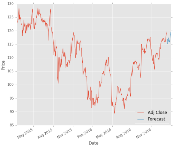
As we can see the blue color showcased the forecast on the stock price based on regression. The forecast predicted that there would be a downturn for not too long, then it will recover. Therefore, we could buy the stocks during the downturn and sell during the upturn.
Future Improvements and Challenges for Stock Analysis
To further analyse the stocks, here are some ideas on how you could contribute. These ideas would be useful to get a more comprehensive analysis of stocks. Feel free to let me know should there be more clarifications needed.
- Analyse economic qualitative factors such as news (news sourcing and sentimental analysis)
- Analyse economic quantitative factors such as HPI of a certain country, economic inequality among the origin of the company
Purpose, Github, Code, and Your Contributions
The purpose of this Proof Of Concepts (POC) was created as a part of the investments side project that I am currently managing. The goal of this application is to help you retrieve and display the right financial insights quickly about a certain company stock price and predicting its value.
In the POC, I used Pandas- Web DataReader to find the stock prices, Scikit-Learn to predict and generate machine learning models, and finally Python as the scripting language. The Github Python Notebook Code can be located here.
Feel free to clone the repository and contribute whenever you have time.
Value Investing with Stock Analysis
In lieu of today’s topics about stocks analysis. You could also visit my Value Investing Publication where I talked about scraping stocks financial information and displaying it in an easy to read dashboard which processes stocks valuation based on Value Investing methodology. Please visit it and contribute 🙂
Acknowledgments
I would like to thank you for my fellow Accountancy and Finance friends who gave me constructive feedback on this publication. I really enjoyed learning that you gained many values from this publication of mine.
Finally… Reach out to me
Whew… That’s it, about my idea which I formulated into writings. I really hope this has been a great read for you guys. With that, I hope my idea could be a source of inspiration for you to develop and innovate.
Please reach out to me via my LinkedIn and subscribe to my Youtube Channel.
Happy coding 🙂
Disclaimer: This disclaimer informs readers that the views, thoughts, and opinions expressed in the text belong solely to the author, and not necessarily to the author’s employer, organization, committee or other group or individual. References are picked up from the list and any similarities with other works are purely coincidental
This article was made purely as the author’s side project and in no way driven by any other hidden agenda.